Probability theory, the section of mathematics devoted to studying and quantifying random processes, has many useful applications to real world systems. Consider a random system where the next state is dependent on the previous state, such as a stock market model where the price of stocks on a given day is dependent on changes in price on the previous day.
Such a random system can be described as a Markov process. Markov processes are used to model a variety of important random systems, “… including communication systems, transportation networks, image segmentation and analysis, biological systems and DNA science analysis, random atomic motion and diffusion in physics, social mobility, population studies, epidemiology, animal and insect migration, queuing systems, resource management, dams, financial engineering, actuarial science, and decision systems. Such processes are named after Andrei Markov, a Russian mathematician whose work on random processes paved the way for the theory of Markov processes.

What Is A Markov Process?

In an abstract setting, consider a system moving through time that has n possible states that is a random process. Such a process is considered to be a first-order Markov process if the state at the next time period is only reliant on the current state of the system. For example, we can model economic mobility in a society as a Markov process, where a person’s probability that they will be in a certain economic class is only dependent on their parents’ economic class.
If the process is a first-order Markov process, then we can assign a transitional probability, t_ij for all i,j in {1,… , n}, where t_ij represents the probability that if a system is currently in state j that it will be in state i at the next time period. Since t_ij is a probability, it must be a value between 0 and 1. Furthermore, since we know that the system will always be in some state with probability 1, it must be the case that for a fixed j, we have

t_1j + t_2j + … + t_nj = 1.We can use the transitional probabilities defined above to create an n by n matrix T = [t_ij]. We call such a matrix the transition matrix or stochastic matrixof the Markov process. The transition matrix can be used to easily compute the probability of the system being in a certain state after a certain period of time. To see that this is the case, let

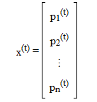
be the state vector of the Markov process at time period t, where p_j^(t) denotes the probability that the system is in state j at time t. We have x^(t+1) = Tx^(t), as this follows from the definition of transitional probabilities and the fact that the process we are considering is a first-order Markov Process. With the previous equation, we can conclude that

x^(t) = Tx^(t-1) = T(Tx^(t-2)) = T²x^(t-2) = … = T^tx⁽⁰⁾.

Hence, the state vector at every time is completely determined by the transitional probabilities and x⁽⁰⁾, which is called the initial state vector.

Example Markov Process

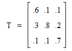
Consider modeling economic mobility in a society as a Markov process. We will have three states: upper, middle, and lower economic classes (indexed by 1, 2 and 3 respectively). Suppose that we conducted a study to discover the probabilities that a family will move up or down in economic class after a generation based on its current economic class. We can encode these probabilities into the following transition matrix:

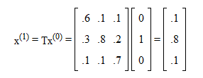
In this example, the probability that a family moves from the lower economic class to the higher economic class over one geneartion is t_1,3= .1. Consider the initial state vector corresponding to starting in the middle class:

After one generation, we have:

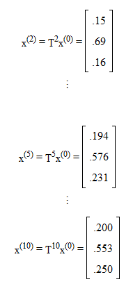
Thus, if a family is currently in the middle economic class, the probability that it will move to the upper economic class after one generation is .1. We can continue the process to discover the probabilities of moving to different economic classes after multiple generations:

Thus, for a family starting in the middle economic class, after 10 generations the probability that the family will be in the upper class is .2, the middle class .553, and the lower class .25. Now consider the initial state vector corresponding to starting in the lower class:

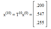
Then we have for x⁽¹⁰⁾:

Thus, for a family starting in the lower economic class, after 10 generations the probability that the family will be in the upper class is .2, the middle class .547, and the lower class .255.
Notice that the system is converging to a certain set of probabilities for social mobility as the number of generations increases. Also, the set of probabilities that the system is converging to appears to be independent of the initial class of the family. We will now formalize these observations.

Regular Markov Processes and Equilibrium

A Markov process is called a regular Markov process if some power of the corresponding transition matrix has only positive elements. It can be shown that every regular Markov process eventually converges to a certain state vector, called the steady-state vector, that is independent of the initial state vector. When a system reaches the steady-state vector, it is considered to be an equilibrium. The equilibrium of Markov processes is an appealing quality of certain real life models, such as population statistics after multiple generations. [2]
Consider the problem of trying to determine the steady-state vector s for a given regular Markov process. We know that Ts = s, since if this is not the case, then the steady-state vector is moving away from the steady-state vector, which is a contradiction. Thus, 1 is an eigenvalue of T with corresponding eigenvector s. Hence, if a Markov process is regular, we can determine the steady-state vector of the process by considering the eigenvector of T corresponding to eigenvalue 1 that is normalized such that the sum of the probabilities is equal to 1. Note that eigenvectors of T corresponding to eigenvalue 1 are unique up to common multiples if T represents a regular Markov process, so there is only one such normalized eigenvector.

Continuing with the above model of social mobility, we have:

which is what was expected from our calculations. Thus, continuing with the social mobility model, this would tell us that after a sufficient number of generations, the probability that a family will be in the upper class is .2, the middle class .55, and the lower class .25, and that these probabilities are independent of the economic class the family started in.
For a simple example of a Markov process that is not regular, consider the Markov process with the following transition matrix:

For the above Markov process, the initial state vector is the state vector of the system at any time, and thus the Markov process does not have a steady-state vector that is independent of the initial state vector. It turns out that, as was the case for the steady-state vector, many important questions about a given Markov process can be recast as questions about the corresponding transitional matrix, and thus problems in probability can be solved using linear algebra techniques.

Further Applications:

So far we have only considered the simplest of Markov processes, first-order discrete-time discrete-state Markov processes. While there are a few real systems that can be accurately described by such processes, such as economic mobility over generations, often times we want to consider continuous-time and continuous-state processes, such as the market value of financial stock options over time. These processes may also depend on more previous states than just the current one to determine future states, and are thus of higher order. As you would expect, Markov processes have been generalized to describe a wide range of physical systems.